1. Terrestrial Laser Scanning in
River Environments
Dr David Hetherington
Ove Arup and Partners, Newcastle upon Tyne, UK.
Tuesday the 1st June 2010
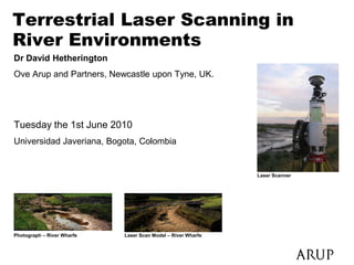
Universidad Javeriana, Bogota, Colombia Laser Scanner
Laser Scanner
Photograph – River Wharfe Laser Scan Model – River Wharfe
2. Presentation Structure
• Spatial Data Theory
• Terrestrial Laser Scanning principles and
operation
• Reflectivity, Time-of-flight measurement, Scanner operation
• Potential uses and example projects
• Example projects, Potential applications, where next?
• Benefits and Limitations
• Fit-for-purpose?
• Questions
4. Processing spatial data into elevation models
• Manual filtering – to remove anomalies
• Ground filtering – to remove lowest or highest
points
• Regularisation / gridding – to allow for surfacing
• Averaging – between surveys
• Lumping – all data together
• Extrapolation – estimating beyond surveys
• Interpolation – predicting lines and data between
points
• ALL OF THESE IMPACT ON DATA QUALITY
8. Survey method and interpolation error
Potential volumetric estimation error for various survey techniques,
and interpolation methods in a river system (from Milan et al,
2007)
10. Terrestrial Laser Scanning (TLS) - types
• Various types exist
• Ultra-short range (hand held static) used in manufacturing,
medicine, archaeology
• Short range (mobile static) used in heritage, archaeology, small
buildings
• Medium range (mobile static) used in buildings, street scenes,
infrastructure.
• Long Range (mobile static) used for large buildings,
townscapes, topographical surveys, mining, forestry.
• Vehicle Based (mobile dynamic) automated survey and data
registration. Used to easily map towns, long roads, motorways
etc.
• All have their relative benefits and weaknesses.
• Choosing the correct method is key
11. Measurement using Laser Scanning –
Basic Principles
• Lidar:
• “Light Detection And Ranging” using a pulsed laser beam.
• Numerous automated measurements = Scanning
• 3 platforms for lidar scanning
• Satellites (extremely long range)
• Airborne (long to moderate range)
• Terrestrial (very short to moderate range)
• All based on time-of-flight principles of laser pulses
• All are reflectorless and non-contact.
• Measurements are based on reflections from physical
surfaces
12. Laser measurement theory - REFLECTIVITY
• 3 types of light reflection:
Diffuse Mirror-like Retro
(most surfaces) (Glass, mirrors flat (roadsigns, bike
water surfaces) reflectors, strips on
high-vis jackets)
13. Time-of-flight measurement
• A laser pulse generator sends out infrared light pulses.
• Reflected echo signals generate a receiver signal.
• Time interval counted by a quartz-stabilised clock frequency.
• The calculated range value is then processed and saved.
14. A simplified lidar scanner
1. Range finder electronics
2. Laser beam
3. Rotating mirror
4. Rotating optical head
5. Connection to Laptop
6. Laptop
7. Software
15. Terrestrial laser scan data
• Range of up to 1500m (for highly reflective surfaces)
• Sub-cm accuracy
• A single scan can contain over 7-million data points
• A single model is made of multiple scans from various
locations to avoid data shadow
• Each coordinate point is associated with colour (as
measured by an integrated camera) and intensity
(reflectivity) information.
• Data and scans are automatically georeferenced using
an integrated GPS system.
• Can be easily linked to thermal imagery cameras.
16. Riegl LMSZ420 laser scanner
• Arup own this model of medium-long range
scanner.
• Time of Flight-based scanner
• Range of around 1km
• Point accuracy of around 10mm (can be reduced to
around 5mm with repeat scanning)
• Allowing for very high resolution point clouds.
• Integrated camera captures colour data
• Captures intensity of return data and attached to
each coordinate (along with colour).
18. Spatial & Temporal Change
1000km
Rates
River scale
slope adjustment
Reach scale
Increasing Spatial Scale
slope adjustment
1km Planform change
Barform change
1m Cross-section
adjustment
Fine sediment
movement
1mm
1 day 1 month 1 year 1000 years 10000 years
Increasing Time Scale
19. Spatial & Temporal Survey
1000km Limits
Aerial Photo's
Airborne
Increasing Spatial Scale
LIDAR
GPS
1km
Theodolite
1m
Photogrametry
1mm
1 day 1 month 1 year 1000 years 10000 years
Increasing Time Scale
20. Spatial & Temporal Survey
1000km Limits
Aerial Photo's
Airborne
Increasing Spatial Scale
LIDAR
GPS
1km
Theodolite
1m
Photogrametry NO DATA
1mm
1 day 1 month 1 year 1000 years 10000 years
Increasing Time Scale
21. 1000km
Lidar limits
Aerial Photo's
Airborne
Increasing Spatial Scale
LIDAR
GPS
1km
Theodolite
1m
Terrestrial LIDAR
Photogrametry NO DATA
1mm
1 day 1 month 1 year 1000 years 10000 years
Increasing Time Scale
22. Multiple scans and overlap
Multiple scans
from various
perspectives
reduce “shadow”
23. Point Cloud Model Creation (merging scans)
• All individual scan need to be registered into one
common coordinate system.
• Various ways to do this..
• Quickest and most reliable way is via “pattern
matching” / “surface matching”.
• I-Site software is a good option.
• Allows for surfaces to be created, cross sections to
be cut, volumes calculated, change/deformation to
be observed.
• Output possible in numebrous formats including
CAD.
24. Example laser scan model – River Wharfe
• 25 High-Resolution Scans
• Scans Merged to within <5mm
• 21 million Data points
• 1 point per cm2
25. Error Measurement On The Wharfe
x y z
Mean -0.0176 0.00011 0.001078
Standard Error 0.002014 0.004054 0.001856
Median -0.013 0 0.001
Standard Deviation 0.015983 0.032429 0.014846
Sample Variance 0.000255 0.001052 0.00022
b 15
10 Rock Gaps
5
0
-1 -0.5 0 0.5 1
c
20
15
10
5
Grass
0
-1 -0.5 0 0.5 1
27. Controlled Experiment Description
• Scans taken at various known distances, heights,
locations, sequences and amounts on and around the
bar.
• Models were merged and processed in various ways
in RiScan Pro, Polyworks and Surfer.
• Models were then tested against a EDM Theodolite
data-based model (appx 3mm accuracy) including 3200
coordinate points within the 8x8 grid.
• EDM data taken systematically across the 8x8 grid in
order to leave surface undisturbed.
• EDM data catagorised as exposed rock tops and
topographic lows.
28. Example results – Gravel scale measurement
Scan height = 1.5m
Scan amount = 1 Mismeasurement errors
Scan locations = n/a
All Highs Lows
Scan distance = 10m
Processing = none Min = 0.000001 0.000001 0.00007
Scan resolution = max Max = 0.121 0.121 0.114
Repeat scans = no
Merging = reflectors only Mean = 0.0243 0.0146 0.0339
29. Example results – Gravel scale Measurement
Mismeasurement errors
Scan height = 1.9m
Scan amount = 2 All Highs Lows
Scan locations = opposite Min = 0.00002 0.00002 0.00016
Scan distance = 20m
Processing = default OCTREE Max = 0.1266 0.1266 0.1124
Scan resolution = max Mean = 0.0270 0.0205 0.03359
Repeat scans = no
Merging = reflectors only
30. Arolla Outwash Plain Study - Description
• To measure geomorphological change on a daily
basis over a 2-week period.
• Net Change and change at a local level.
• 12 scans were taken between 5AM and 11AM at zero-
low flow after overnight re-freezing of glacier water.
• AIMS
• To test the appropriateness of TLS for such a project.
• To better understand geomorphological change at small
temporal intervals over a number of spatial scales.
• To monitor the gravel resource on the plain
• To better manage extraction for building purposes and
downstream sedimentation.
44. Scope of work
• To describe, assess and understand the
geomorphological system
• To monitor the site and habitat geomorphology
during and post construction
Challenges for measurement and understanding
• Complex morphology (a result of tidal, fluvial and geotechnical
processes)
• Tides
• Operational plant and machinery
• Structurally complex over many scales
• Potential for widespread and subtle change
• Difficult to measure due to ground conditions and available
perspective
45. Geomorphological
Assessment
• Desk Study
• Walk over survey using
customised pro-forma
• Separated the channel
into process units on
each bank based on key
characteristics and
process evidence
• Noted features within
each process unit
(gullies, shear faces, cut
banks, failures)
• Quantify Morphology..?
60. Survey Description - Nenthead
• Scan surveys completed on 07/10/03 and
16/08/04 (approx 10 months)
• One season of high Discharges
• Concentrated on main unstable slope
(approximately 80% of sediment source area)
• 1st survey no reflectors – 2nd survey with
reflectors
• 5 scan positions (only 2 used)
• Surveys linked using common points between
models in RiScan
68. Volumetric change
Slope Change Volume Channel Change Volume
(m3) (m3)
Positive Volume 11.63 Positive Volume 29.10
[Deposition]: [Deposition]:
Negative Volume 77.57 Negative Volume 33.32
[Erosion]: [Erosion]:
Net Volume [Cut- - 75.94 Net Volume [Cut- - 4.22
Fill]: Fill]:
• Approximately 80 m3 of sediment removed from the local system
over a 9 month period.
• One high flow season
• Efficient channel – steep and high energy
69. Downstream engineering works
R. Nent engineered to stabilize mine spoil through
Village of Nenthead.
Series of pools and blockstone rapids created
Pools act as sediment traps
70. Engineering works model flood hydraulics
700
600
500
400
74 cross-
300
200
sections
100
0
0 100 200 300 400 500 600 700 800 900 1000
Flood shear Fine sed threshold Coarse sed threshold
20cumec flood simulated using HEC RAS model
Distinct pool-rapid hydraulic shear stress fluctuation
Sub 2mm material just movable in pools
Coarser material likely to be trapped in pools
71. Deposition downstream
Exceedence percentage
120
100
80
60
40
20
0
0.1 1 10 100 1000
Clast size (mm)
POOL 1 POOL 2 POOL 3
Coarse material in pool 1
Fining in downstream pools
72. Deposition downstream
Conventional EDM
survey
Deposition measured in
upstream 3 pools up to 2002
Deposition reduced in upper
pool but continuing in pools 2
and 3 up to 2004
190m3 sediment deposited in
the pools
Roughly matches the 2 x 80m3 removed from
mine slopes
74. Ulley Dam – Emergency monitoring
• Used to remotely monitor the dam face during a
failure event (movement above 2mm would be
detected)
• Also used to measure water surface area for draw-
down calculations
75. Valley Tidal Doors – Asset Measurement
• Used to produce digital document of a historical asset and a wider
DEM and bare-earth DTM.
79. Practical Considerations: Water
Return to scanner
Diffuse reflection from valley side
Scan direction
Water surface
(mirror-like)
reflection
3D Model: 3 scans (high resolution)
81. Measuring Water Surface variations
Study Aims and Objectives
LMSZ210 – Older Model Scanner
360deg horizontal
90deg vertical
5mm accuracy
0.0025deg angular resolution
8000-12000 points are acquired/second
350m radial range
Non destructive
Rapid
•This study utilises terrestrial LiDAR data to map water surface
character based on the local standard deviation of the laser returns.
•A revised biotope unit classification is proposed and tested using
similar data from an upland river in the UK.
83. Data Collection 1
•Biotope units were visually identified by the survey team and mapped
using theodolite survey
•Retro reflectors mapped using theodolite survey
•Sites scanned using TLS
84. Data Collection 2
•Automatic retro-reflector recognition and scan registration in RiScan Pro™
•Data captured inside the wetted perimeter of the channel were extracted
manually
•Data exported as ASCII files for input and analysis using the SURFER™
surface mapping software
85. Data Analysis
•The local standard deviation of the data were computed using a 0.2 m radius
moving window
•Data were gridded at 0.04 m so as to capture the smallest biotope unit seen
at the study sites
•Local standard deviation values at each of the measured biotope locations
were then extracted from the grids using the residual function in SURFER™
•Local standard deviation values interrogated at each known biotope location
•Statistical properties of each biotope determined
86. Results: Temporal variation
•Temporal data from the River Skirfair at Arncliffe reveal that the median
surface roughness values for the recorded biotopes are generally
consistent between scans.
•Suggests that local surface standard deviation is a robust measure
recording consistent values at the same biotope locations
•The surface expression of each biotope is subject to minimal temporal
variation and should therefore be definable.
87. Results: Spatial consistency
•Between river roughness values show good consistency particularly
around the median values recorded for each river.
•These data allow physical surface roughness limits to be defined for
each biotope that can then be used to map the biotope distribution along
scanned river reaches.
88. Results: Spatial consistency
•Min stdev Max stdev
Pool 0 0.005
Accelerating flow 0.012 0.016
Glide 0.016 0.02
Deadwater 0.018 0.02
Chute 0.019 0.023
Eddy 0.023 0.025
Run 0.023 0.025
Riffle 0.025 0.03
Cascade 0.035 0.046
Boil 0.036 0.039
Unbroken standing wave 0.046 0.05
Broken standing wave 0.05 0.09
•Clear from the data that the local roughness variability
shows considerable overlap between biotope units
suggesting that the present classifications are overly
complex
89. Results: Spatial consistency
•Units may be usefully amalgamated to •Five roughness sub-divisions are
form a broader set of flow types. proposed, amalgamating:
Pools and deadwater zones
Accelerating flow areas
Riffles runs chutes and glides
Rapids cascades
Boils and Waterfalls
90. Results: Typology validation
frequency biotope successfully
Unit descriptor classified frequency amalgamated biotope successfully classified
Run 0.00 0.90
Glide 0.14 0.75
Chute 0.20 0.59
Rapid 0.38 1.00
Riffle 0.25 0.55
Deadwater 0.71 0.71
Pool 1.00 1.00
91. Experiment - Conclusions
Despite issues of signal loss due to absorption and transmission
through the water the reflected signal generates an extremely detailed
and accurate objective map of the water surface roughness which may
be compared to known biotope locations as defined by visual
identification in the field.
Biotope surface roughness delineation has proved problematic using
the current set of biotopes found in the literature due to large within
biotope surface variation. This suggests an overly complex set of
biotope classifications.
The results also suggest that present biotope classifications are overly
complex and could reasonably be reduced to three or four
amalgamated units.
92. Where next…………?
• Sediment size measurement
160
140 a
120 2
R = 0.9653 b
100
c
80
2 Linear (a)
R = 0.9202
60
Linear (c)
40
20 y = 1.0876x - 3.5613 Linear (b)
R2 = 0.9711
0
0 10 20 30 40 50
1000
Sediment size (mm)
wolman
100
laser all
10
0 20 40 60 80 100
% excedence
93. Problems with TLS and Fitness-for-purpose
• An inappropriate measurement technique
when:
• mm or sub-mm accuracy is required on key
points.
• Only one distance measurement is needed
• No appropriate vantage is available
• The measurement area exceeds a practical
limit (around 10km2)
• Water is present (not always a problem)
• Point interpolation error is accepted
94. Key considerations
• TLS is not the answer to all measurement problems
• When it is the appropriate it is extremely useful
• Try to consider different types of TLS
• Cost reduction and “added value” in Arup?
• It can reduce risk and thus benefit H&S
• The technology is improving
• Could one survey provide many different types of
information? (dimensions, change, hydraulics, habitat, roughness,
colour, reflectivity, sediment size, vegetation characteristics)
95. Key Considerations
• An ideal technique when:
• Good accuracy and point resolution is required
over medium to large areas
• (<+/-1cm error over 10m2 up to 10s of km2)
• There is no access but good vantage (non-contact
tool)
• The data are required for multiple purposes
• Measurement and monitoring, GIS, Virtual
Reality
• The scene of measurement is complex and
includes features such as vegetation, overhangs,
wells and bridges.
96. TLS – Warnings and Benefits
• What are the implications / uses of a survey?
• Control?
• State expected data character, nature and utility early.
• Sometimes overboard and can be over sold.
• It can be “the ultimate” data set.
• Allows errors to be tracked and understood.
• Can measure more than just topography.
• Great in Emergencies.
• Its getting better …..